See what really
drives your
portfolio’s risk.
A few holdings can carry most of the risk. Start with a simple example, then explore how assumptions, market shocks and withdrawals change the picture.
€750 one-time session · Free interactive examplesNo account or holdings upload required

40% of the capital.
How much of the risk?
This example holds four asset classes. Equities account for 40% of the money. Their share of portfolio risk may surprise you.
Hypothetical example. Risk means contribution to annual portfolio volatility under the stated covariance assumptions.
Explore portfolio risk.
Understand the trade-offs.
Portfolio construction connects asset weights to risk, return assumptions, cash flows and decision rules. Use these free interactive tools to compare allocations, inspect risk contributions and test the assumptions behind a decision. Start with the question that matters to you.
The approach: mandate / evidence / policy
Capital has a job. The allocation must answer to the horizon, liquidity needs and constraints.
Change the assumption that matters. Ask whether the decision survives a plausible alternative.
Decide what would trigger a review before a difficult market forces the question.
Two portfolios.
The same market test.
A different allocation changes the exposures you carry into a difficult market. Compare two portfolios under identical, explicit shocks. Then trace the difference to the assets that caused it.
Four asset classes · Same shocks · Full attribution
Calculating the allocation difference…
One scenario never tells the whole story.
Select a row to inspect its shocks and attribution. A and B use the same weights in every row.
| Constructed scenario | Portfolio A | Portfolio B | B minus A |
|---|
These examples have no assigned probabilities. Higher returns in one scenario do not establish a better allocation.
Inspect the shocks, portfolio weights & calculation
The presets include falling and rising markets to make the trade-off visible in both directions. These are deliberately constructed one-period scenarios, not historical episodes, forecasts or assigned probabilities. Edit any of the four asset shocks to create a custom scenario (−100% to +100% per asset). Each shock applies once to starting asset weights: portfolio return = Σ(weight × asset shock). Attribution = (weight B − weight A) × asset shock, so the four contributions sum exactly to return B − return A. No within-period rebalancing, fees, taxes, currency conversion or cash flows are modelled.
Annual volatility is a separate model estimate, calculated using the fixed baseline covariance in experiment 03. It is not a forecast of the selected scenario’s loss. Selecting the current experiment 03 allocation follows its weights; its correlation toggle does not change this desk’s baseline covariance. No portfolio is ranked as universally better. Display values are rounded; CSV export preserves calculation precision.
| Asset | Weight A | Weight B | Asset shock | B − A contribution |
|---|
Which exposure would you be willing to hold through this outcome—and what evidence would make you change it?
Inspect the sources of riskChange an estimate.
Test the allocation.
An optimizer treats the inputs you give it as the basis for its decision. Compare a model that uses the changed return estimate directly with one that blends it with a starting assumption and stabilises the covariance matrix.Try this Move the return adjustment in both directions. Watch how much capital each model reallocates.
A change in the estimate, not a market move. All other asset-return assumptions stay fixed.
Set the last two controls to 100% and 0% to make the models identical.
Hover to inspect. Click to set the assumption, or use the arrow keys on the chart.Tap the plot to set the assumption. Use the slider above for precise adjustments.
Loading the experiment…
Inspect the allocation, inputs & calculation
Hypothetical annual returns: equities 7.5%, government bonds 3.5%, credit 5%, gold 4%. Annual volatilities: 18%, 7%, 11%, 15%. Risk-aversion coefficient A = 4. The same long-only, fully invested utility objective is used in both models.
Utility = w′μ − (A/2)w′Σw. Search over a 2.5-percentage-point weight grid; results are discretised examples, not continuous-solver optima. Allocation moved = half the sum of absolute weight changes. The regularised matrix blends the original covariance with its diagonal. The return anchor blends the changed estimate with the unchanged prior. This is an explicit teaching model, not a full Black-Litterman implementation or data-estimated Ledoit-Wolf intensity.
| Asset class | Unanchored baseline | Unanchored now | Anchored baseline | Anchored now |
|---|
The line connects grid evaluations at 0.25 pp intervals. It illustrates sensitivity, not future performance or proof that a method is universally superior.
Before changing an estimate. A more stable allocation can be useful. It can also react too slowly to genuine information. The question is how much confidence the evidence deserves—not which line looks smoother.
Next questionHow much weight should a conviction carry?See how a view updates a market-implied starting point.Express a view.
Decide how much to trust it.
Suppose you expect equities to outperform government bonds. Express that return difference, then decide how strongly it should update the starting assumptions.Try this Move confidence from 0% to 100%. Watch the returns and allocation respond to the same view.
A hypothetical annual return difference. The prior implies — before your view is introduced.
Confidence controls the strength of the update. It is not a probability that the view will be correct.
Loading the Bayesian update…
Inspect the Bayesian update, allocation & inputs
This is a computed, single-relative-view Black–Litterman example. Equilibrium excess returns are π = δΣw, using δ = 4 and a hypothetical reference portfolio 40 / 30 / 20 / 10. A 2% risk-free rate is added to all total-return estimates. The view vector is P = [1, −1, 0, 0]; τ = 0.05.
For 0 < c < 1, view uncertainty is Ω = ((1−c)/c)τPΣP′. The limiting updates at c = 0 and c = 1 are calculated directly. Posterior excess returns are π + cΣP′(Q−Pπ)/(PΣP′). The optimizer uses predictive covariance Σ + τΣ − cτΣP′PΣ/(PΣP′). The mean, the view and confidence are illustrative, not independently estimated investment inputs.
| Asset class | Prior return | Posterior return | No-view weight | Posterior weight |
|---|
A view can affect assets outside the pair because covariance links their returns. Confidence does not establish forecasting skill. This example is independent of experiment 01’s simpler return anchor.
Before acting on a conviction. Expressing a view is easy. Justifying the confidence—and recognising what would invalidate it—is the harder part of portfolio construction.
Next questionWhere does the portfolio’s risk actually sit?Compare the money invested with the risk each exposure contributes.What you own.
What drives your risk.
Capital weights tell you where the money is invested. Risk contributions show how each exposure contributes to portfolio volatility under the model’s assumptions.Try this Choose equal capital weights, then switch to converging correlations. Equal investments need not mean equal sources of risk.
Moving one weight redistributes the remaining capital proportionally. Total allocation stays at 100%.
Each cell shows the assumed correlation between two asset classes.
Loading the experiment…
Inspect the risk decomposition & assumptions
Euler contribution to volatility: RCᵢ = wᵢ(Σw)ᵢ / σₚ. The bars show RCᵢ / σₚ. Signed contributions sum to 100%; a negative contribution would indicate a diversifying position under this model, not a negative capital weight.
Baseline correlations are illustrative and fixed. “Converging” blends the baseline covariance 50/50 with a perfectly positively correlated covariance having the same individual volatilities. The blend preserves positive semidefiniteness. It changes correlations only; it is not a calibrated crisis forecast.
| Asset class | Capital weight | Risk contribution | Annual volatility input |
|---|
Before calling a portfolio diversified. More holdings do not automatically mean more independent sources of risk. Start with the relationships and the contribution each position makes to the whole.
Next questionWhat changes when you start withdrawing?Follow the same returns in a different order.Same returns.
A different retirement.
Two portfolios experience exactly the same 20 annual returns, in opposite orders. Remove withdrawals and their ending values match. Add withdrawals and the order becomes consequential.Try this Keep withdrawals on, then switch them off. With no withdrawals, the two ending values coincide.
Fixed nominal amount, withdrawn at each year-end after that year’s return. No inflation adjustment, taxes, fees or new contributions.
Sorted from lowest to highest for the early-loss path; reversed for the late-loss path. This deliberately isolates the effect of ordering.
This is a deterministic illustration. Neither path is assigned a probability.
Loading the experiment…
Inspect the annual paths & calculation
Starting capital = €100,000. Each year: available = previous wealth × (1 + return); actual withdrawal is the smaller of the requested amount and available capital. Remaining wealth is floored at zero. A depleted path stays at zero. “Withdrawn” reports actual cash paid, not requested withdrawals that could not be funded.
The returns are a constructed teaching sequence, not historical observations or simulation draws. The example does not estimate a safe withdrawal rate. With no cash flows, terminal wealth is W₀ × ∏(1 + rₜ), which is independent of return order.
| Year | Early return | Early capital | Late return | Late capital |
|---|
Before funding withdrawals. A retirement plan needs explicit withdrawal and review rules. An average return alone cannot describe the path an investor must live through.
Next questionHow much does the risk model leave out?Compare a bell curve with a model that allows heavier tails.The same volatility.
A different bad case.
A bell curve and a fat-tailed model can share the same theoretical mean and variance while telling different stories about severe losses. Compare 20,000 reproducible synthetic one-year returns for the allocation in the risk experiment.Try this Keep volatility fixed and lower the degrees of freedom. Compare the average loss in the worst 5% of outcomes.
Change the volatility of both distributions together. Return means stay fixed.
Each Student-t draw is scaled by √((ν−2)/ν) so its theoretical variance matches the Gaussian model.
Tail statistics use the entire sample. Shading marks each model’s worst 5%. The full chart includes overflow in endpoint bins; the tail view omits returns above μ − σ. All percentages use the entire sample.
Comparing the distributions…
Inspect the simulation, tail definitions & reproducibility
20,000 independent one-year arithmetic return draws per model; deterministic seed 20261015. The mean follows the selected source: experiment 01’s changed return inputs for its linked allocations, experiment 02’s posterior returns for its linked allocation, or unchanged base returns for standalone presets and custom weights. Volatility comes from experiment 03’s selected covariance, multiplied by the scale. It does not include the Black–Litterman posterior’s parameter covariance.
For standard normal Z and independent U ∼ χ²(ν), normal return = μ + σZ; Student-t return = μ + σZ√((ν−2)/U). Both have the same theoretical mean and variance. Finite-sample moments differ, especially at small ν. Common Z draws reduce comparison noise; they do not make the distributions equal.
VaR-95 is the loss at the 1,000th worst return (nearest-rank cutoff). Expected shortfall is minus the mean of the worst 1,000 returns. Losses are expressed as positive percentages; a negative loss means a gain. These are one-period statistical approximations, not wealth paths: their unbounded lower tails can produce returns below −100%. No clipping is applied to improve appearances.
| Statistic | Gaussian | Student-t |
|---|
Before trusting a risk number. A precise loss number is conditional on a distribution. Comparing models shows how much of your apparent certainty comes from that choice.
Next questionHow do these findings become a plan?See the decisions a written investment mandate needs to record.Five questions.
One decision process.
Take the question that matters to you into the underlying research. Each article explains the method, its assumptions and its limits, with equations and references for a closer examination.
An allocation is
not yet a plan.
A model can propose weights. Your investment mandate must connect those weights to the life they are intended to fund—and the constraints you actually face.
Purpose & risk capacity
Your objectives, horizon, liquidity needs and capacity to hold through losses.
Cross-border implementation
Account structure, fund domicile, currency and implementation costs for your circumstances.
Rules for changing course
Concentration limits, rebalancing thresholds and the circumstances that trigger a review.
The Strategic Session brings these decisions into a written Investment Policy Statement and strategic allocation. You retain custody and implement through your own broker.
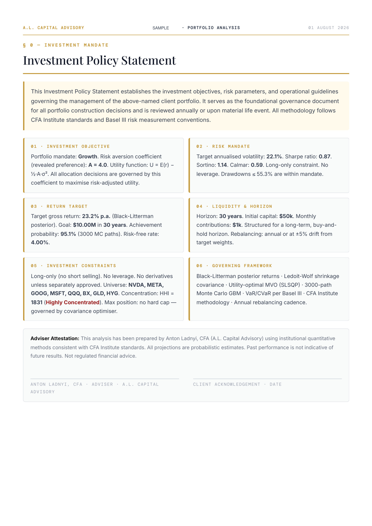
The mandate: objectives, risk parameters, liquidity and investment constraints, recorded together.
Pages from the sample report. Figures describe that example, not the interactive models above or expected client results.What the numbers
cannot promise.
The framework is useful only when its limits are visible. More decimal places do not resolve uncertainty, and a more complex model does not automatically produce a better decision.
Estimates are conditional.
Risk and return estimates depend on the sample, the model and the regime. A displayed optimum is an answer to stated assumptions.
Stability has a trade-off.
Anchoring and regularisation can reduce sensitivity. They can also suppress useful information. Simpler allocations remain meaningful benchmarks.
These are experiments.
The examples use hypothetical asset classes. They do not assess your circumstances, select securities or forecast your investment outcome.
Understand the model.
Then question it.
These are educational portfolio construction tools by Anton Ladnyi, CFA. The examples use four hypothetical asset classes: equities, government bonds, credit and gold. They use constructed assumptions, not live holdings or market forecasts.
What is the difference between allocation weight and risk contribution?
Allocation weight is the share of capital invested in an asset. Risk contribution measures how that asset contributes to portfolio volatility, accounting for its weight, volatility and correlations with the other assets. In this page’s opening example, equities hold 40% of capital but contribute approximately 72.7% of modelled volatility. That result belongs to the stated assumptions; it is not a general rule for a 40% equity portfolio.
Inspect the risk contribution toolHow does the portfolio stress test work?
The comparison desk applies the same asset-class return shocks to both portfolios. Each portfolio’s scenario return is the sum of its asset weights multiplied by those shocks. The difference is attributed asset by asset. Scenarios are constructed examples, not historical backtests or probabilities, and exclude fees, taxes, trading and rebalancing.
Worked example: the same shocks, two allocations
For the comparison desk’s “Growth shock” scenario, the default balanced allocation is 40% equities, 30% government bonds, 20% credit and 10% gold. The equity-heavy alternative uses 70%, 10%, 15% and 5% respectively.
| Asset class | Shock | Balanced weight | Equity-heavy weight |
|---|---|---|---|
| Equities | −30% | 40% | 70% |
| Government bonds | +5% | 30% | 10% |
| Credit | −15% | 20% | 15% |
| Gold | +10% | 10% | 5% |
Balanced portfolio: −12.50%. Calculation: 0.40 × (−30%) + 0.30 × 5% + 0.20 × (−15%) + 0.10 × 10%.
Equity-heavy portfolio: −22.25%. Its loss is 9.75 percentage points larger under these shocks. This illustrates exposure differences, not an expected return, likelihood or investment recommendation.
What do the five experiments calculate?
The assumptions tool compares long-only allocations on a 2.5 percentage-point weight grid with anchoring and covariance shrinkage. The conviction tool uses a single relative Black–Litterman view. The risk tool uses Euler contributions to volatility. The withdrawal tool reverses a fixed 20-year return sequence. The tail tool compares 20,000 seeded Gaussian and variance-normalised Student-t draws using 95% Value at Risk and Expected Shortfall.
Model definitions and relevant assumptions are shown beside each experiment. Displayed precision does not imply forecast accuracy.
Can these tools recommend my portfolio?
No. The tools do not collect your holdings, assess suitability or select securities. Their purpose is to help you understand dependencies and formulate better questions. A personal investment mandate also needs your objectives, time horizon, liquidity, loss capacity and implementation constraints.
See how a model connects to an investment mandateFor the full equations, research references and model-governance discussion, read the original portfolio construction working paper. Explore the focused guides to Black–Litterman, covariance shrinkage, Expected Shortfall and Monte Carlo simulation.
Foundational reading: Black and Litterman’s Global Portfolio Optimization (1992) and Ledoit and Wolf’s Honey, I Shrunk the Sample Covariance Matrix (2004). These papers motivate the methods; the simplified teaching implementations and their limits are documented above.
Interactive edition published . Author: Anton Ladnyi, CFA. The original working paper was published in February 2026. No account or holdings upload is required to use the experiments.
Explore the equations, assumptions and references behind the tools. Download the PDF or visit the original research edition.